C# Backpropagation Tutorial Xor

Content

• Only One Neuron A Linear Model
• Activation Functions!
• Time For Battle With A Genetic Algorithm
• Not The Answer You’re Looking For? Browse Other Questions Tagged Machine

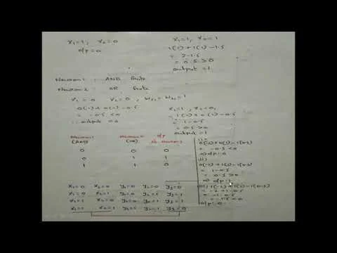
These branch off and connect with many other neurons, passing information from the brain and back. Millions of these neural connections exist throughout our bodies, collectively referred to as neural networks. Notice in the output, our genetic algorithm advances in fitness as the populations evolve. After 2,000 epochs, our best brain had a fitness of 3.99. When we run the network, we get a very correct answer. All ouputs are 0 or less, except for 1 AND 1, which provides an output of 0.99, which when rounded is 1.

If a straight line or a plane can be drawn to separate the input vectors into their correct categories, the input vectors are linearly separable. If the vectors are not linearly separable, learning will never reach a point where all vectors are classified properly. However, it has been proven that if the vectors are linearly separable, perceptrons trained adaptively will always find a solution in finite time.

Only One Neuron A Linear Model

Above parameters are set in the learning process of a network (Fig.1). For example, there is a problem with XOR function implementation. “Activation Function” is a function that generates an output to the neuron, based on its inputs. Although there are several activation functions, I’ll focus on only one to explain what they do. Neural networks are a type of program that are based on, very loosely, a human neuron.

The training technique used is called the perceptron learning rule. The perceptron generated great interest due to its ability to generalize from its training vectors and learn from initially randomly distributed connections.

The most fit of these networks can go on to create even more precise networks, until we have a satisfactory solution to the problem at hand. As shown above, the larger an input vector p, the larger its effect on the weight vector w. Thus, if an input vector is much larger than other input vectors, the smaller input vectors must be presented many times to have an effect.

We’ll fill in the helper functions, including the fitnessFunction in a moment, but first a few notes on the above code. Notice that we’ve replaced the neural network training section with a genetic algorithm training method. We instantiate the genetic algorithm with a crossover of 50%, mutation rate of 1%, population size of 100, epoch length of 2,000 iterations, and the number of weights at 12. While the other numbers are variable, the last number is not. This one must match the exact number of weights used in your neural network. This gives us a total of 12 variable weights for the network. Our genetic algorithm will take care of assigning the weights.

Activation Functions!

In fact, this was the first neural network problem I solved when I was in grad school. TensorFlow is an open-source machine learning library designed by Google to meet its need for systems capable of building and training neural networks and has an Apache 2.0 license. ANN is based on a set of connected nodes called artificial neurons . Each connection between artificial neurons can transmit a signal from one to the other. The artificial neuron receiving the signal can process it and then signal to the artificial neurons attached to it. This happened because when you calculate the delta error for back-propagation, you used the output of the dot product and not the output of the activation function. With these deltas, we can get the gradients of the weights and use these gradients to update the original weights.

To calculate the gradients, we use the cache values from the forward propagation. Now let’s build the simplest neural network with three neurons to solve the XOR problem and train it using gradient descent. This structure of neurons with their attributes form a single-layer neural network.

Time For Battle With A Genetic Algorithm

XOR is a classification problem and one for which the expected outputs are known in advance. It is therefore appropriate to use a supervised learning approach. The XOR gate consists of an OR gate, NAND gate and an AND gate. If an XOR gate has more than two inputs, then its behavior depends on its implementation. In the vast majority of cases, an XOR gate will output true if an odd number of its inputs is true.

Biases are added to shift the values within the activation function. If you made it this far we’ll have to say THANK YOU for bearing so long with us just for the sake of understanding a model to solve XOR. If there’s just one take away we hope it’s that we don’t have to be a mathematician to start with machine learning. The function simply returns it’s input without applying any math, so it’s essentially the same as using no activation function at all. We’ve open sourced it on GitHub with the hope that it can make neural networks a little more accessible and easier to learn.

Thinking about creating the next HAL, Data, or Terminator? You just need to devise the correct fitness function with a larger neural network. Of course, while the total capabilities of the neural network aren’t fully realized yet, it’s certainly possible to push the boundaries of science. Whenever you create a fitness function for a genetic algorithm, remember that the most important part is to provide a fine gradient score. No matter how good or bad a network is, you should be able to give some numeric indication of how far off the network is from success.

Not The Answer You’re Looking For? Browse Other Questions Tagged Machine

This is done by measuring the accuracy of the network after a period of training. On the contrary, the function drawn to the right of the ReLU function is linear. Applying multiple linear activation functions will still make the network linear. For the XOR problem, 100% of possible data examples are available to use in the training process.

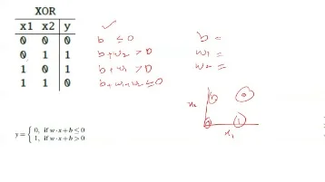
• The basic idea is to take the input, multiply it by the synaptic weight, and check if the output is correct.
• The closer the resulting value is to 0 and 1, the more accurately the neural network solves the problem.
• This gives us a total of 12 variable weights for the network.
• As shown above, the larger an input vector p, the larger its effect on the weight vector w.

In the hidden layers, the lines are colored by the weights of the connections between neurons. Blue shows a positive weight, which means the network is using that output of the neuron as given. An orange line shows that the network is assiging a negative weight. Within a column, we have all the features as rows. Next, we call the initialize_parameters function to initialize the weights.

In our recent article on machine learning we’ve shown how to get started with machine learning without assuming any prior knowledge. We ended up running our very first neural network to implement an XOR gate. The purpose of this article is to create a sense of understanding for the beginners, on how neural network works and its implementation details. The next post in this series will feature a implementation of the MLP architecture described here, including all of the components necessary to train the network to act as an XOR logic gate. A limitation of this architecture is that it is only capable of separating data points with a single line.

It looks like my initial choice of random weights has a big impact on my end result after training. The accuracy (i.e. error) of my neural net is varying a lot depending on my initial choice of random weights. I’m trying to understand what would be the best neural network for implementing an XOR gate.

Neural networks are one of the methods for creating artificial intelligence in computers. They are a way of solving problems that are too difficult or complicated to solve using traditional algorithms and programmatic methods. Some believe that neural networks are the future of computers and ultimately, humankind. Set epochs to 1, so that train goes through the input vectors just one time. It allows you to pick new input vectors and apply the learning rule to classify them. If a bias is not used, learnp works to find a solution by altering only the weight vector w to point toward input vectors to be classified as 1 and away from vectors to be classified as 0. This results in a decision boundary that is perpendicular to w and that properly classifies the input vectors.